Real-Time Point-by-Point Forecasts on the ATP World Tour

Predicting the outcome of sports has always been a fascinating topic for me, and having been an avid tennis fan since the age of 11, I have been obsessed with the prospect of forecasting tennis results. Now, I am happy to say that I have built a prototype that can predict the odds of all best-of-3 ATP World Tour matches in real time.

This master project has been a long time coming. Last year, I used match-level tennis data to predict match/tournament outcomes at the beginning of each match / round. A few weeks ago, I used detailed point-by-point data on the ATP World Tour to calculate the chance that a men's professional player would win a best-of-3 match from any scoreline. To me, predicting win odds in real-time just seemed like a natural progression that exhibited further granularity in my tennis predictions.

To see real-time predictions of tennis matches, you can follow my Github project site here. This blog post will focus on outlining the methodology of my model. As a data scientist, I have explored and learned most of these advanced techniques on my own, and am always open to feedback on how this prediction model can be improved.

The Mathematical Model

When planning my methodology, it immediately became clear to me that my model had to contain Bayesian elements.

 In other words, my model had to incorporate substantial prior / domain knowledge of tennis win probabilities, before real tennis data can be used to update our model and reflect a more informed result. The reason for this is two-fold:

(1) I wanted the model to make intuitive sense in nearly all (if not all) cases. For instance, if a player wins a point, his chances of winning should go up. If a player loses a game, his chances of winning should most definitely go down.

(2) While I had six years (2010-2015) worth of point by point tennis data, it actually is not enough to use it as a source of truth. A tennis match contains thousands of different situations, and after splitting the point-by-point data into these various states, each match situation on average only contained fewer than 100 observations. As a result, putting too much emphasis on this raw data may cause my model to generate non-sensical results (e.g. winning a point may lead to a lower winning percentage)

The Underlying Distribution of the Tennis Prediction Model

To create an initial model that incorporated substantial tennis knowledge, I broke a tennis match down to its component parts. From a simplistic point-level view, a player's fate in a match consists of two key statistics:

• His chance of winning a point while serving
• His chance of winning a point while returning.

Assuming that each point is independent, we can generate an entire backward dynamic programming problem, where each state denotes a particular point situation (e.g. 1 set all, 2-3 in games, serving at 40-15), and the end states are final scores that already the winner/loser (e.g. a 6-3, 6-4 scoreline). Solving the problem recursively allows us to have a "base win probability" at each stage of a match that can be tweaked for each particular matchup.

The graph below describes how match win probabilities fluctuate given various serve win and return win probabilities as discussed above.

The average win % when serving and returning is 65% and 35% respectively on the ATP World Tour, which is why I chose a range between those two values (55-75%) and (25-45%). We also notice in this graph that different serve and return % lead to the same winning percentages. For the sake of simplicity, I decided to use only the serve/return % that deviated the same amount from the tour average (e.g. 64/34, 70/40 etc.), which is essentially a diagonal cross section of the surface above. The resulting graph looks like this:

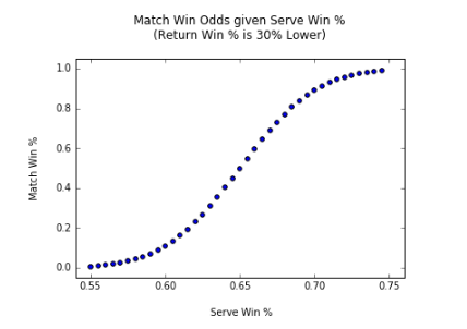
As anticipated, this graph goes to 0 to 1 on both tails fairly quickly. This makes sense, since a player with a significant serve/return advantage can easily dominate a match in tennis.

So how do we use these findings to create our initial model? After all, we should be choosing different serve/return probabilities for different matchup situations. For instance, world number 1 Novak Djokovic should have a higher serve and return win % when playing against a player outside of the Top 100 player then when he plays against Roger Federer.

As a result, I created a grid that summarizes the match win probabilities grouped by ranking buckets:

These odds are based on a combination of my past experience following tennis closely for the past 10 years and a detailed look at various statistics on the ATP World Tour site (player records against Top 10, lowest ranked players top players have lost, etc.)

With this table, we can now find the serve win % in the graph above that is equal the match win % in the grid, determine the return win % from that (which we defined as 30% lower), and plug it back into our backward dynamic programming model, which outputs the match win percentage at any tennis scoreline. These "base win probabilities" will serve as our initial model for our tennis predictions.

Updating the Model with Match-Specific Data

With the base model in place, we seek to examine factors that can help us adjust / make our probability predictions with more certainty. The factors that I decided upon, based on my tennis knowledge, are:

• Court Surface - Different surfaces lead to vastly difference service win and return win percentages. Clay courts, a slower surface, tend to lead to longer rallies, which neutralizes service advantages. Thus, service win % is typically lower and return win % is usually higher. Grass courts, on the other hand, is a faster surface that augments the service advantage. As a result, players who lead (i.e. are service breaks up) in a grass court match tend to a higher chance of winning the match compared to other surfaces.

• Recent Form - Performance in recent events should be incorporated for a match-specific scenario. While the base model already puts player rankings into account, rankings only reflect player performance in the past 12 months. It makes sense to introduce a factor that puts more weight on results in the past 3 months, as momentum is known to play a factor in tennis results.

• Head-to-Head Record - It is important to also account for the head-to-head record of a specific match. Some players are known to have problems playing particular opponents, (think Nadal vs. Davydenko, or Federer vs. Nalbandian for instance), so these instances should be accounted for.

• Actual Point-by-Point Odds - Since our initial model was based on intuition, we should tweak the model using actual match win probabilities by every scoreline from actual ATP World Tour matches. Even though there are on average less than 100 observations per scoreline, it is still valuable to incorporate this information to ensure real-life accuracy.

• Actual Ranking Win Odds - Our initial model also made some intuitive assumptions about how often players did against opponents of various ranking groups. Again, it's important to incorporate real match information and tweak our models accordingly.

Combining and Fine-Tuning Our Model

Combining these different factors requires us to define our initial probability estimate from our base model (let's call it p) as a random variable with a designated distribution, so that we can update the parameters of this distribution as we take on new data based on the specific matchup scenario. Since we are estimating the probability of a player winning / losing, which is essentially a Bernoulli variable with parameter p, it is most mathematically efficient to designate p to follow a Beta Distribution. 

A Beta Distribution has two parameters a, b - they dictate what the distribution of p looks like between 0 or 1. If a is larger than b, then p's distribution is more concentrated to 1. If b is larger than a, then p's distribution is more concentrated to 0. The larger a and b are, the tighter (i.e. more certain) the distribution is. Here are examples of what the distribution looks like with various a's and b's:

Beta Distribution Graphs courtesy of Matt Bognar, Ph.D of University of Iowa. See his application here.

The reason why depicting our win estimate p as a Beta Distribution is mathematically efficient is that updating the distribution with new information involves merely adding parameters a and b proportionally. For instance, if you have 10 new matches, 7 of which led to wins, you can merely update a, b with a+7, b+3 respectively. Such efficiency is due to the fact that the Beta Distribution is a conjugate prior of a Bernoulli likelihood function. You can learn more about this here.

To fine-tune our model, we need to figure out how much we should weigh our base model and the match-specific criteria detailed above. To do so, we train our model using match data from 2010-2014, and test our model using match data from 2015. Since our model predicts probabilities, we then split our 2015 test data into 20 buckets by the estimated probabilities (matches that were predicted to have a 0-5% win chance, 5-10%, 10-15% etc.) For each bucket, we calculate the % of matches that resulted in victories and determined whether this proprotion matched the probability denoted by that bucket. The graph below represents the results of our best fitted model:

Each blue dot represents the actual percent of matches that were victories, each red line depict the probability bucket range and each green line represents the confidence interval range that is deemed acceptable given the number of samples in the bucket. While some of the blue dot estimates somewhat deviate from what the bucket should represent, all of them are still within the green range. Upon inspecting other parameters, we found this set of parameters that displayed this graph to be the most appropriate model to use. 

The parameters in this model imply that the base probability model governs the majority of the prediction (magnitude 100), followed by ranking and head-to-head factors (magnitude 10). Other factors such as surface, recent form and actual point-by-point odds are less significant (magnitude 5).

Making the Predictions Real Time

With the model in place, we used scoreboard.com and web scraping techniques to obtain tennis score lines in real time. These scores are then automatically fed into the model, which stores past odds and updates the new odds. The following graphs are examples of what our live dashboard looks like over time.

And there we have it - version 1.0 of my real-time point-by-point match predictions of all ATP World Tour matches. Suggestions? Feedback? Questions? Please feel free to comment below.

Note: Credit for the tennis point-by-point goes to Jeff Sackmann's Github account. You can find all sorts of cool tennis-related data there.